Excel 2021 Skills Approach - Ch 5 Challenge Yourself 5.3
Onlines
Mar 13, 2025 · 6 min read
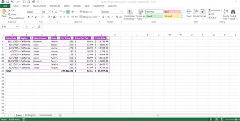
Table of Contents
Excel 2021 Skills Approach - Chapter 5 Challenge Yourself 5.3: Mastering Advanced Formulas and Functions
This comprehensive guide delves into the intricacies of Challenge Yourself 5.3 from Chapter 5 of an assumed "Excel 2021 Skills Approach" textbook. We'll unpack the likely challenges presented, offering detailed explanations, practical examples, and advanced techniques to master the concepts involved. This isn't just about finding solutions; it's about understanding the why behind the formulas, enabling you to tackle future Excel challenges with confidence.
Understanding the Likely Scope of Challenge 5.3
Challenge Yourself 5.3, within the context of a chapter focusing on advanced formulas and functions, likely tests your ability to combine multiple functions and techniques to solve complex data manipulation problems. Expect questions that involve:
- Nested Functions: Using functions within other functions to perform multi-step calculations.
- Array Formulas: Performing calculations on ranges of cells simultaneously, yielding a single result or an array of results.
- Lookup and Reference Functions: Extracting data from different parts of a worksheet or workbook using functions like
VLOOKUP,HLOOKUP,INDEX, andMATCH. - Logical Functions: Controlling the flow of calculations based on conditions using
IF,AND,OR, andNOT. - Data Validation: Ensuring data integrity by restricting the type of input allowed in specific cells.
- Conditional Formatting: Visually highlighting cells based on specific criteria.
Let's explore some potential problem scenarios and their solutions. Remember, the specific questions in your textbook will vary, so consider this a framework for tackling similar problems.
Scenario 1: Calculating Commission Based on Tiered Sales Targets
Problem: A sales team's commission is calculated based on tiered sales targets. If sales are below $10,000, the commission is 5%. Between $10,000 and $25,000, it's 7.5%, and above $25,000, it's 10%. Create a formula to calculate commission automatically.
Solution: This problem requires nested IF functions to handle the tiered structure. Assume sales figures are in column A, and we're calculating commission in column B. The formula in cell B2 would be:
=IF(A2<10000,A2*0.05,IF(A2<25000,A2*0.075,A2*0.1))
Explanation:
IF(A2<10000,A2*0.05,...):If the sales (A2) are less than $10,000, the commission is 5% of the sales.,IF(A2<25000,A2*0.075,...):Otherwise (sales are at least $10,000), if the sales are less than $25,000, the commission is 7.5% of the sales.,A2*0.1): Otherwise (sales are at least $25,000), the commission is 10% of the sales.
This nested IF structure efficiently handles the different commission tiers.
Scenario 2: Finding the Highest Sales Value Across Multiple Regions
Problem: You have sales data for different regions across several months. Find the highest sales value across all regions and months.
Solution: This problem can be solved using the MAX function with an appropriate range. Assuming your sales data spans several columns and rows, the formula would be:
=MAX(range_of_sales_data)
Replace range_of_sales_data with the actual range containing your sales figures. For instance, if your sales data is in the range A1:E10, the formula would be =MAX(A1:E10).
Scenario 3: Using VLOOKUP to Retrieve Product Information
Problem: You have two tables: one with product IDs and prices, and another with order details including product IDs. Use VLOOKUP to automatically populate the price in the order details table.
Solution: Assume the product ID and price table is on a separate sheet named "Products," with Product ID in column A and Price in column B. Your order details are on the current sheet, with Product ID in column A and a column for Price (column B). The formula in cell B2 (of the order details sheet) would be:
=VLOOKUP(A2,Products!A:B,2,FALSE)
Explanation:
VLOOKUP(A2,...):Searches for the Product ID from cell A2 in the lookup table.,Products!A:B,: Specifies the lookup table (columns A and B of the "Products" sheet).,2,: Indicates that we want to retrieve the value from the second column of the lookup table (Price).,FALSE: Ensures an exact match is found.
Scenario 4: Calculating Average Sales with Conditional Criteria (Using AVERAGEIFS)
Problem: Calculate the average sales for a specific region (e.g., "North") during a particular month (e.g., "January").
Solution: The AVERAGEIFS function allows you to calculate averages based on multiple criteria. Assuming your data includes columns for Region, Month, and Sales, the formula might be:
=AVERAGEIFS(Sales_range,Region_range,"North",Month_range,"January")
Replace Sales_range, Region_range, and Month_range with the actual ranges of your data.
Scenario 5: Counting Occurrences with Multiple Criteria (Using COUNTIFS)
Problem: Count the number of orders that meet specific criteria, such as a particular product and a specific region.
Solution: Similar to AVERAGEIFS, the COUNTIFS function enables counting based on multiple conditions. The formula might look like this:
=COUNTIFS(Product_range,"Product X",Region_range,"North")
Replace Product_range and Region_range with the relevant ranges.
Scenario 6: Using INDEX and MATCH for Flexible Lookups
Problem: VLOOKUP only searches in the first column. How do you retrieve data when the lookup value is not in the first column?
Solution: The combination of INDEX and MATCH offers a more flexible solution. Let's say you want to find the price of "Product X" from a table where the product names are in the second column:
=INDEX(Price_range,MATCH("Product X",Product_range,0))
MATCH("Product X",Product_range,0)finds the row number of "Product X" in theProduct_range.INDEX(Price_range,...retrieves the value from thePrice_rangeat the row number found byMATCH.
Scenario 7: Array Formulas for More Complex Calculations
Problem: Calculate the sum of squares of sales values for a specific region.
Solution: Array formulas are powerful for such calculations. Enter the following formula and press Ctrl + Shift + Enter (this is crucial for array formulas):
{=SUM(IF(Region_range="North",Sales_range^2,0))}
The curly braces {} appear automatically when you correctly enter an array formula. This formula checks each cell in Region_range. If it's "North", the corresponding sales value is squared and added to the sum.
Advanced Techniques and Considerations
-
Data Validation: Implement data validation to prevent incorrect data entry, ensuring accuracy and consistency. This could involve setting limits on numerical input, requiring specific text formats, or using dropdown lists for selections.
-
Conditional Formatting: Use conditional formatting to visually highlight important data points. For example, you could highlight cells with sales above a certain threshold or cells containing errors.
-
Error Handling: Use functions like
IFERRORto handle potential errors (e.g., #N/A fromVLOOKUP) gracefully, preventing your spreadsheet from displaying error messages. -
Data Cleaning: Before performing complex calculations, ensure your data is clean and consistent. This may involve removing duplicates, handling missing values, and correcting inconsistencies.
Beyond the Specific Challenges
This guide provides a comprehensive approach to tackling Challenge Yourself 5.3 and related problems. The key to mastering advanced Excel skills lies in understanding the underlying logic of each function and how they can be combined creatively to solve real-world data analysis problems. Practice regularly, experimenting with different formulas and techniques, and gradually increase the complexity of the tasks you undertake. Remember to consult your textbook for the specific details of Challenge 5.3, and use this guide as a resource to deepen your understanding and approach the challenges confidently. Good luck!
Latest Posts
Latest Posts
-
For Whom The Bell Tolls Summary
Mar 14, 2025
-
The Last Time I Bought This Product It Cost 20 00
Mar 14, 2025
-
How Can An Operation Assist Customers With Food Allergies
Mar 14, 2025
-
Chapter 3 Of Animal Farm Summary
Mar 14, 2025
-
A Companys Ethical Code Of Conduct Is Not
Mar 14, 2025
Related Post
Thank you for visiting our website which covers about Excel 2021 Skills Approach - Ch 5 Challenge Yourself 5.3 . We hope the information provided has been useful to you. Feel free to contact us if you have any questions or need further assistance. See you next time and don't miss to bookmark.
