Each Of The Following Graphs Shows A Hypothetical Relationship
Onlines
Mar 18, 2025 · 6 min read
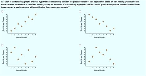
Table of Contents
Decoding Hypothetical Relationships: A Deep Dive into Graph Interpretation
Graphs are powerful visual tools that help us understand and represent relationships between different variables. Whether it's the correlation between ice cream sales and temperature or the impact of advertising spend on website traffic, graphs provide a concise and readily interpretable summary of complex data. This article will explore the art of interpreting hypothetical relationships depicted in various graph types, focusing on identifying trends, drawing inferences, and understanding the limitations of visual representations. We'll move beyond simple observation to analyze underlying patterns and consider potential causal relationships.
Understanding the Basics: Types of Graphs and Their Applications
Before diving into hypothetical relationships, it's crucial to understand the common types of graphs used to represent data. Each graph type has its strengths and weaknesses, making some more suitable than others for depicting specific kinds of relationships.
1. Scatter Plots: Unveiling Correlations
Scatter plots are ideal for visualizing the relationship between two continuous variables. Each point on the plot represents a data point, with its horizontal position indicating the value of one variable and its vertical position indicating the value of the other. The pattern of points reveals the correlation between the variables:
- Positive Correlation: Points cluster along a line sloping upwards from left to right, indicating that as one variable increases, the other tends to increase as well. Example: Height and weight.
- Negative Correlation: Points cluster along a line sloping downwards from left to right, indicating that as one variable increases, the other tends to decrease. Example: Hours spent sleeping and hours spent studying (for a certain student).
- No Correlation: Points are scattered randomly, indicating no apparent relationship between the variables. Example: Shoe size and intelligence.
- Nonlinear Correlation: Points follow a curve rather than a straight line, suggesting a more complex relationship. Example: The relationship between the amount of fertilizer used and crop yield (too much fertilizer can be detrimental).
Interpreting hypothetical scatter plots requires careful consideration of:
- Strength of Correlation: How tightly clustered are the points around a potential line of best fit? A tighter cluster indicates a stronger correlation.
- Outliers: Are there any data points significantly distant from the main cluster? Outliers can skew the interpretation and warrant further investigation.
- Causation vs. Correlation: A strong correlation does not necessarily imply causation. While a strong correlation suggests a possible causal link, other factors could be at play.
2. Line Graphs: Tracking Changes Over Time
Line graphs are best suited for showing changes in a variable over time. The x-axis represents time, while the y-axis represents the value of the variable. Line graphs effectively highlight trends:
- Increasing Trend: The line slopes upwards, indicating an increase in the variable over time.
- Decreasing Trend: The line slopes downwards, indicating a decrease in the variable over time.
- Constant Trend: The line is relatively flat, indicating little or no change in the variable over time.
- Cyclical Trend: The line shows regular fluctuations, repeating a pattern over time.
When interpreting hypothetical line graphs, consider:
- Rate of Change: How steep is the slope of the line? A steeper slope indicates a faster rate of change.
- Turning Points: Are there any points where the trend changes direction (e.g., from increasing to decreasing)? These inflection points are often significant.
- External Factors: Could external events or interventions have influenced the observed trend?
3. Bar Charts and Histograms: Comparing Categories and Distributions
Bar charts are used to compare the values of a categorical variable across different categories. Histograms, on the other hand, display the distribution of a continuous variable. Both are useful for identifying patterns and differences:
- Bar Charts: The height of each bar represents the value of the variable for a particular category.
- Histograms: The height of each bar represents the frequency of data points falling within a specific range.
Analyzing hypothetical bar charts and histograms requires attention to:
- Scale of the Axes: The scale used can influence the perception of differences. Be mindful of potentially misleading scales.
- Category Representation: Ensure categories are clearly defined and mutually exclusive.
- Data Distribution: Histograms reveal the shape of the data distribution (e.g., normal, skewed).
4. Pie Charts: Showing Proportions
Pie charts are effective for illustrating the proportions of different categories within a whole. Each slice represents a category, and its size reflects its proportion to the total.
When interpreting hypothetical pie charts, note:
- Percentage Labels: Clear percentage labels are crucial for easy interpretation.
- Visual Distortion: Be aware that slight differences in slice sizes can be visually exaggerated.
Analyzing Hypothetical Relationships: A Case Study Approach
Let's examine some hypothetical scenarios and illustrate how to analyze the relationships depicted in graphs.
Scenario 1: The Impact of Advertising Spend on Sales
Imagine a scatter plot showing the relationship between advertising expenditure and sales revenue. A strong positive correlation would suggest that increased advertising spend is associated with higher sales. However, this does not automatically prove causation. Other factors, such as product quality, market competition, and seasonal variations, could also influence sales.
Scenario 2: The Effect of Sleep Deprivation on Performance
A line graph could depict the effect of sleep deprivation on cognitive performance over several days. A downward trend in performance as sleep deprivation increases would suggest a negative correlation. This would support the hypothesis that insufficient sleep impairs cognitive function.
Scenario 3: Consumer Preferences for Different Product Features
A bar chart could show the distribution of consumer preferences for different product features (e.g., price, quality, design). The height of each bar indicates the popularity of each feature. This visualization helps identify which features are most valued by consumers.
Scenario 4: The Distribution of Ages in a Population
A histogram could display the age distribution of a population. The shape of the histogram (e.g., whether it's symmetrical or skewed) provides valuable insights into the population's demographic structure.
Beyond Visual Interpretation: Statistical Analysis
While visual inspection of graphs provides valuable insights, a more rigorous approach often involves statistical analysis. Statistical tests can help determine the strength and significance of correlations, assess the probability of observing the data by chance, and quantify the relationship between variables.
Techniques like correlation coefficients (e.g., Pearson's r) measure the strength and direction of linear correlations. Regression analysis helps model the relationship between variables and predict outcomes. These quantitative methods enhance the interpretation of hypothetical relationships and provide a more robust foundation for drawing conclusions.
The Importance of Critical Thinking
Interpreting hypothetical relationships depicted in graphs requires critical thinking skills. It's essential to consider the following:
- Data Source and Methodology: How was the data collected? Are there any biases or limitations in the data collection process?
- Scale and Units: Are the scales on the axes appropriate? Are the units of measurement clearly defined?
- Context and Background: What is the context of the data? What other factors might be relevant?
- Limitations of Visual Representation: Graphs can be misleading if not presented carefully. Be wary of distorted scales or selective presentation of data.
By carefully considering these aspects, you can develop more accurate and nuanced interpretations of hypothetical relationships.
Conclusion
Graphs are indispensable tools for understanding relationships between variables. However, interpreting these relationships requires more than just a cursory glance. A deep understanding of graph types, careful consideration of potential biases, and the incorporation of statistical analysis are crucial for drawing accurate and meaningful conclusions from hypothetical data. Always remember that correlation does not equal causation, and critical thinking remains paramount in the process of interpreting visual representations of data. By applying these principles, we can unlock the power of graphs to reveal valuable insights and guide informed decision-making.
Latest Posts
Latest Posts
-
A Wall Of Fire Rising Summary
Mar 18, 2025
-
Highway Hypnosis Is Related To
Mar 18, 2025
-
Amoeba Sisters Video Recap Protists And Fungi Answer Key
Mar 18, 2025
-
Chapter Summaries For Tale Of Two Cities
Mar 18, 2025
-
Hesi Chronic Kidney Disease Case Study
Mar 18, 2025
Related Post
Thank you for visiting our website which covers about Each Of The Following Graphs Shows A Hypothetical Relationship . We hope the information provided has been useful to you. Feel free to contact us if you have any questions or need further assistance. See you next time and don't miss to bookmark.
