Match Each Graph With The Corresponding Function Type
Onlines
Mar 22, 2025 · 7 min read
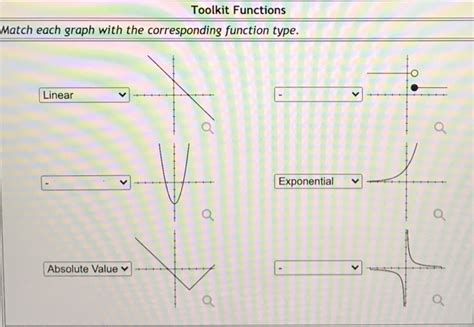
Table of Contents
Matching Graphs with Function Types: A Comprehensive Guide
Understanding the relationship between a graph and its corresponding function type is fundamental to success in algebra, calculus, and beyond. This comprehensive guide will walk you through various function types, their characteristic graph shapes, and key features to help you confidently match graphs with their equations. We'll explore linear, quadratic, cubic, polynomial, rational, exponential, logarithmic, trigonometric, and piecewise functions, providing clear examples and explanations.
Linear Functions (f(x) = mx + b)
Linear functions are characterized by their straight-line graphs. The equation is in the form f(x) = mx + b, where 'm' represents the slope (rate of change) and 'b' represents the y-intercept (the point where the line crosses the y-axis).
Key Features:
- Constant Slope: The slope 'm' is constant throughout the line. A positive slope indicates an upward trend, a negative slope indicates a downward trend, and a slope of zero indicates a horizontal line.
- Straight Line: The graph is always a straight line.
- Y-intercept: The y-intercept 'b' is the point where the line intersects the y-axis (x=0).
Identifying a Linear Function Graph:
Look for a straight line. If the graph is a straight line, it represents a linear function. You can determine the slope by finding the rise over run between any two points on the line. The y-intercept is the point where the line crosses the y-axis.
Example: A graph showing a straight line with a positive slope and a y-intercept of 2 represents the function f(x) = 2x + 2.
Quadratic Functions (f(x) = ax² + bx + c)
Quadratic functions are represented by parabolas—U-shaped curves. The general form is f(x) = ax² + bx + c, where 'a', 'b', and 'c' are constants.
Key Features:
- Parabola Shape: The graph is a parabola, either opening upwards (if a > 0) or downwards (if a < 0).
- Vertex: The vertex is the highest or lowest point on the parabola.
- Axis of Symmetry: A vertical line that divides the parabola into two symmetrical halves. Its x-coordinate is given by -b/(2a).
- x-intercepts (Roots): The points where the parabola intersects the x-axis (where f(x) = 0). These can be found using the quadratic formula or factoring.
Identifying a Quadratic Function Graph:
Look for a U-shaped curve. The direction of the parabola (upward or downward) indicates the sign of 'a'. The vertex represents the minimum or maximum value of the function. The x-intercepts are the points where the parabola crosses the x-axis.
Example: A parabola opening upwards with a vertex at (1, -2) and x-intercepts at x = 0 and x = 2 could represent a function such as f(x) = x² - 2x.
Cubic Functions (f(x) = ax³ + bx² + cx + d)
Cubic functions are represented by curves with at most two turning points. The general form is f(x) = ax³ + bx² + cx + d, where 'a', 'b', 'c', and 'd' are constants.
Key Features:
- S-shaped Curve: The graph typically resembles an S-shape.
- At most two turning points: These are points where the graph changes from increasing to decreasing or vice-versa.
- One or three x-intercepts: The points where the curve intersects the x-axis.
Identifying a Cubic Function Graph:
Look for an S-shaped curve with at most two turning points. The number of x-intercepts can vary.
Example: A graph showing an S-shaped curve with one x-intercept at x = 1 and two turning points could represent a function similar to f(x) = (x-1)³.
Polynomial Functions (f(x) = aₙxⁿ + aₙ₋₁xⁿ⁻¹ + ... + a₁x + a₀)
Polynomial functions are the generalization of linear, quadratic, and cubic functions. They have the form f(x) = aₙxⁿ + aₙ₋₁xⁿ⁻¹ + ... + a₁x + a₀, where 'n' is a non-negative integer (the degree of the polynomial), and the 'aᵢ' are constants.
Key Features:
- Smooth curves: Polynomial functions produce smooth, continuous curves without any breaks or sharp corners.
- Number of turning points: A polynomial of degree 'n' can have at most (n-1) turning points.
- Number of x-intercepts: A polynomial of degree 'n' can have at most 'n' x-intercepts.
Identifying a Polynomial Function Graph:
Look for smooth curves with a number of turning points consistent with the degree of the polynomial.
Example: A graph with four x-intercepts and three turning points would likely be a quartic (degree 4) polynomial function.
Rational Functions (f(x) = P(x) / Q(x))
Rational functions are of the form f(x) = P(x) / Q(x), where P(x) and Q(x) are polynomial functions and Q(x) is not the zero polynomial.
Key Features:
- Asymptotes: Rational functions often have asymptotes—lines that the graph approaches but never touches. These can be vertical asymptotes (where the denominator is zero) or horizontal asymptotes (describing the behavior as x approaches positive or negative infinity).
- Discontinuities: There might be points where the function is undefined (vertical asymptotes or holes).
Identifying a Rational Function Graph:
Look for graphs with asymptotes and possible discontinuities. Vertical asymptotes occur where the denominator is zero. Horizontal asymptotes describe the end behavior of the function.
Example: A graph with a vertical asymptote at x = 2 and a horizontal asymptote at y = 1 suggests a rational function such as f(x) = (x+1)/(x-2).
Exponential Functions (f(x) = aᵇˣ)
Exponential functions have the form f(x) = aᵇˣ, where 'a' is a positive constant (a ≠ 1) and 'b' is a positive constant (b ≠ 1).
Key Features:
- Rapid Growth or Decay: Exponential functions exhibit rapid growth (if b > 1) or decay (if 0 < b < 1).
- Horizontal Asymptote: There's a horizontal asymptote at y = 0 (unless a vertical shift is involved).
- Always Positive: The function is always positive (unless a vertical shift is involved).
Identifying an Exponential Function Graph:
Look for a curve that shows rapid growth or decay and approaches a horizontal asymptote.
Example: A graph that rapidly increases and approaches the x-axis as x becomes increasingly negative represents an exponential growth function.
Logarithmic Functions (f(x) = logₓ(y))
Logarithmic functions are the inverse of exponential functions. They have the form f(x) = logₓ(y), where x is the base and y is the argument.
Key Features:
- Inverse Relationship to Exponential Functions: The graph is a reflection of the corresponding exponential function across the line y = x.
- Vertical Asymptote: There is a vertical asymptote at x = 0 for the function f(x) = logₓ(x)
- Increasing or Decreasing: The function is increasing if the base is greater than 1 and decreasing if the base is between 0 and 1.
Identifying a Logarithmic Function Graph:
Look for a curve that is a reflection of an exponential function and has a vertical asymptote.
Example: A graph showing a curve that increases slowly and approaches a vertical asymptote at x = 0 represents a logarithmic function with a base greater than 1.
Trigonometric Functions (sine, cosine, tangent, etc.)
Trigonometric functions (sine, cosine, tangent, cosecant, secant, cotangent) describe the relationships between angles and sides of triangles and have periodic behavior.
Key Features:
- Periodicity: The graphs repeat their values at regular intervals (periods).
- Amplitude (for sine and cosine): The distance between the maximum and minimum values.
- Asymptotes (for tangent and cotangent): Vertical asymptotes occur at certain values of x.
Identifying Trigonometric Function Graphs:
Look for periodic wave-like graphs. The shape (sine, cosine, tangent, etc.) will determine the specific function.
Example: A graph showing a wave that oscillates between -1 and 1 with a period of 2π represents a sine or cosine function.
Piecewise Functions
Piecewise functions are defined differently over different intervals of their domain.
Key Features:
- Multiple Definitions: The function's rule changes based on the input value.
- Discontinuities: Piecewise functions can have discontinuities where the different parts of the function meet.
Identifying a Piecewise Function Graph:
Look for graphs consisting of different function types combined across different intervals. There might be breaks or discontinuities where the pieces join.
Example: A graph that is a straight line for x < 0 and a parabola for x ≥ 0 represents a piecewise function.
This guide provides a solid foundation for matching graphs with their corresponding function types. Remember to focus on key features like slope, intercepts, asymptotes, turning points, and periodicity to accurately identify the function represented by a given graph. Practice identifying these features in various graphs to solidify your understanding. With consistent practice and attention to detail, you'll become proficient in connecting graphs and their underlying functions.
Latest Posts
Latest Posts
-
Cat On Hot Tin Roof Characters
Mar 23, 2025
-
Amoeba Sisters Video Recap Answer Key Cell Transport
Mar 23, 2025
-
One Concern Voiced By Critics Of Globalization Is That
Mar 23, 2025
-
Estimate The Following Limit Using Graphs Or Tables
Mar 23, 2025
-
Which Of The Following Is True Regarding Bls
Mar 23, 2025
Related Post
Thank you for visiting our website which covers about Match Each Graph With The Corresponding Function Type . We hope the information provided has been useful to you. Feel free to contact us if you have any questions or need further assistance. See you next time and don't miss to bookmark.
