The Graphs Below Depict Hypothesized Population Dynamics
Onlines
Apr 01, 2025 · 6 min read
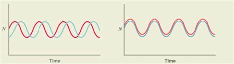
Table of Contents
The Graphs Below Depict Hypothesized Population Dynamics: A Deep Dive into Ecological Relationships
The following analysis delves into the intricate world of population dynamics, interpreting hypothetical scenarios presented through graphical representations. Understanding these dynamics is crucial for comprehending ecological processes, predicting future trends, and informing conservation efforts. We'll explore various factors influencing population growth and decline, considering both intraspecific (within-species) and interspecific (between-species) interactions. This exploration will encompass different models, including exponential growth, logistic growth, predator-prey relationships, and competitive interactions. Remember, these are hypothetical graphs, illustrating general principles rather than representing specific real-world data.
Understanding Population Growth Models: Exponential vs. Logistic
Before interpreting the hypothetical graphs, it's essential to establish a foundational understanding of key population growth models.
Exponential Growth: Unbridled Expansion
Exponential growth, represented by a J-shaped curve, depicts a population increasing at a constant rate. This occurs when resources are abundant, and there are no limiting factors hindering reproduction or survival. The equation often used to model this is: dN/dt = rN, where:
- dN/dt represents the rate of population change over time.
- r is the per capita rate of increase (birth rate minus death rate).
- N is the population size.
While theoretically possible for short periods, exponential growth is rarely sustainable in the long term. Environmental limitations, such as resource depletion, eventually constrain population growth.
Logistic Growth: The Reality of Limits
Logistic growth, represented by an S-shaped curve, incorporates the concept of carrying capacity (K). Carrying capacity represents the maximum population size an environment can sustain indefinitely, given available resources. As the population approaches K, the growth rate slows down, eventually leveling off. The logistic growth equation is more complex: dN/dt = rN((K-N)/K).
This model is more realistic than exponential growth because it acknowledges the influence of environmental limitations on population size. Fluctuations around K are common, reflecting the dynamic interplay between resources, environmental conditions, and population density.
Hypothetical Graph Interpretations: Scenarios and Analyses
Let's now consider various hypothetical graphs depicting different population dynamics scenarios. We will analyze the factors likely driving the observed patterns. Remember, these are simplified representations; real-world population dynamics are far more complex and often influenced by multiple interacting factors.
Scenario 1: The J-curve – Uninhibited Exponential Growth
(Hypothetical Graph: A J-shaped curve showing a steep upward trajectory.)
This graph depicts a classic example of exponential growth. The population increases dramatically over time without apparent limitations. This could represent a scenario where:
- A newly introduced species finds abundant resources in a new environment with minimal competition or predation.
- A species experiencing a sudden surge in resources (e.g., increased food availability due to favorable climatic conditions).
- A species with a high reproductive rate in an environment that can temporarily support rapid growth.
However, this unsustainable pattern will eventually be affected by resource limitations, disease outbreaks, or increased competition, leading to a shift towards a more realistic growth pattern.
Scenario 2: The S-curve – Logistic Growth with Carrying Capacity
(Hypothetical Graph: An S-shaped curve showing rapid initial growth followed by a leveling off as it approaches a carrying capacity.)
This graph illustrates logistic growth, demonstrating the influence of carrying capacity. The initial rapid growth phase mirrors exponential growth, but the rate slows as the population approaches the carrying capacity. This indicates that:
- Resource availability is a limiting factor. As the population grows, competition for resources intensifies, leading to increased mortality or reduced reproductive success.
- Density-dependent factors are influencing population size. These factors, such as disease, competition, and predation, become more significant as population density increases.
- The environment's carrying capacity has been reached (or approached). The population size stabilizes around K, reflecting the sustainable population size for the given resources.
Scenario 3: Predator-Prey Interactions – Cycles of Abundance and Scarcity
(Hypothetical Graph: Two curves, one representing the predator population and the other the prey population, showing oscillating patterns. The predator curve lags behind the prey curve.)
This graph demonstrates the cyclical relationship between predator and prey populations. Notice how:
- Prey population booms first, providing ample food for the predators.
- Predator population then increases, driven by the abundance of prey.
- As predators increase, they exert greater pressure on the prey population, leading to a decline in prey numbers.
- This decline in prey subsequently causes a reduction in the predator population, due to limited food resources.
- The cycle then repeats. The oscillatory pattern reflects the ongoing interaction between predator and prey, with each population influencing the other's dynamics.
Scenario 4: Interspecific Competition – Resource Partitioning and Niche Differentiation
(Hypothetical Graph: Two curves representing populations of two competing species. Initially, both show rapid growth, but one species eventually outcompetes the other, leading to a decline in the latter’s population.)
This graph highlights interspecific competition, where two or more species compete for the same limited resources. We can infer that:
- The species with a competitive advantage (perhaps through superior resource acquisition or tolerance to environmental conditions) eventually dominates.
- The less competitive species experiences a decline in population size, either due to displacement or reduced reproductive success.
- Resource partitioning might occur if the species can adapt to exploit different resources or utilize them at different times. This could lead to coexistence, rather than complete exclusion.
- Niche differentiation can also contribute to coexistence, where species specialize in slightly different aspects of the environment.
Scenario 5: Environmental Impacts – Population Bottlenecks and Recoveries
(Hypothetical Graph: A curve showing a sudden, dramatic decline in population size followed by a slow recovery.)
This graph demonstrates the impact of environmental disturbances on population size. The sudden drop represents a population bottleneck, possibly caused by:
- A natural disaster (e.g., wildfire, flood).
- Disease outbreak.
- Habitat destruction.
- Human intervention.
The subsequent slow recovery demonstrates the challenges of population rebuilding after a significant loss. The rate of recovery depends on factors such as reproductive rate, resource availability, and the severity of the bottleneck. Genetic diversity might also be compromised, impacting the long-term viability of the population.
Beyond the Graphs: Factors Influencing Population Dynamics
While these hypothetical graphs illustrate fundamental concepts, it's crucial to remember that real-world population dynamics are significantly more complex. A myriad of factors can influence population size and growth, including:
- Climate change: Altering temperature, precipitation patterns, and extreme weather events can dramatically impact populations.
- Disease: Outbreaks can decimate populations, particularly if they affect vulnerable age groups.
- Human activity: Habitat destruction, pollution, hunting, and fishing all exert substantial pressure on populations.
- Genetic factors: Inbreeding depression and limited genetic diversity can reduce a population's resilience to environmental changes.
- Stochastic events: Random events, such as unexpected weather patterns or catastrophic events, can significantly affect population size.
Conclusion: The Importance of Understanding Population Dynamics
Understanding population dynamics is essential for effective conservation strategies, resource management, and predicting the long-term impacts of environmental change. By analyzing population trends and the factors influencing them, we can develop strategies to protect endangered species, manage invasive species, and ensure the sustainable use of natural resources. The hypothetical graphs presented here serve as a starting point for exploring this fascinating and complex field. Further research into specific species, ecosystems, and the intricate interplay of biotic and abiotic factors will provide a deeper understanding of the dynamics governing life on Earth. Remember that these simplified models offer a framework; real-world scenarios are significantly richer and require nuanced analysis.
Latest Posts
Latest Posts
-
Shadow Health Gastrointestinal System Hourly Rounds
Apr 02, 2025
-
La Familia Search A Word Answer Key
Apr 02, 2025
-
What Do Larry Page And Jessica Jackley Have In Common
Apr 02, 2025
-
14 1 Practice Three Dimensional Figures And Cross Sections Answers
Apr 02, 2025
-
Cell Membrane And Transport Worksheet Answers
Apr 02, 2025
Related Post
Thank you for visiting our website which covers about The Graphs Below Depict Hypothesized Population Dynamics . We hope the information provided has been useful to you. Feel free to contact us if you have any questions or need further assistance. See you next time and don't miss to bookmark.
